GLS, MMRM, and Power
Power for MMRM
We use the power calculation formula of Lu, Luo and Chen (2008) for Mixed Models of Repeated Measures, which accomodates general missing data patterns. This formula is implemented in the longpower package. We also verify the formula with a simple simulation.
Load packages
library(longpower)
library(nlme)
library(mvtnorm)
library(parallel)
library(ggplot2)
library(contrast)
Simulation settings
gls_sigma <- 2
gls_weights <- c(1, 1.5, 1.75, 2.0)
placebo_mean <- c(0, 0, 0, 0)
active_mean <- c(0, 1, 1.5, 1.8)
retention <- c(1, 0.9, 0.8, 0.7)
# compound symmetric R
R <- matrix(0.5, nrow = 4, ncol = 4)
diag(R) <- 1
N <- 200
Analytic calculations
power.mmrm(power=0.80, ra = retention, Ra=R, N=N, sigmaa = gls_sigma*gls_weights[4])##
## Power for Mixed Model of Repeated Measures (Lu, Luo, & Chen, 2008)
##
## n1 = 100
## n2 = 100
## retention1 = 1.0, 0.9, 0.8, 0.7
## retention2 = 1.0, 0.9, 0.8, 0.7
## delta = 1.798283
## sig.level = 0.05
## power = 0.8
## alternative = two.sidedpower.t.test(power=0.80, n = N/2*retention[4], sd = gls_sigma*gls_weights[4])##
## Two-sample t test power calculation
##
## n = 70
## delta = 1.907529
## sd = 4
## sig.level = 0.05
## power = 0.8
## alternative = two.sided
##
## NOTE: n is number in *each* groupThe t-test delta is larger, which is expect given the conservative handling of the assumed retention rate. The MMRM makes use of partial informatin from dropouts.
Set up data for simulation
dd0 <- expand.grid(time = as.factor(1:4), id = 1:N)
dd0$Time <- as.numeric(dd0$time)
dd0$trt <- ifelse(dd0$id <= N/2, 0, 1)
dd0 <- as.data.frame(model.matrix(~ -1+id+trt*time+Time, data = dd0))
dd0[,'trt:time1'] <- with(dd0, trt*time1)
dd0$Trt <- as.factor(dd0$trt)
dd0$time <- as.factor(dd0$Time)
dd0$Y0[dd0$trt==1] <- as.matrix(subset(dd0, trt==1, c('trt:time1', 'trt:time2',
  'trt:time3', 'trt:time4'))) %*% active_mean
dd0$Y0[dd0$trt==0] <- as.matrix(subset(dd0, trt==0, c('time1', 'time2',
  'time3', 'time4'))) %*% placebo_mean
ggplot(dd0, aes(x=Time, y=Y0, color=Trt)) + geom_line()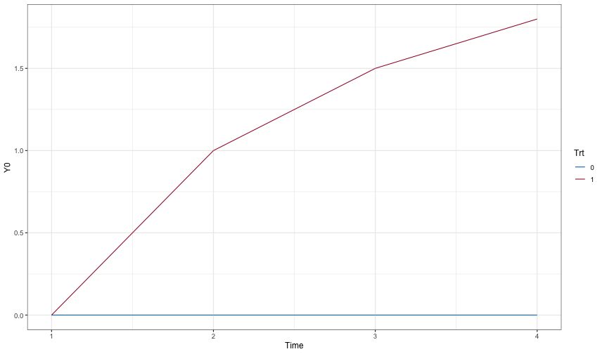
set.seed(20130318)
dd1 <- merge(dd0, data.frame(id = 1:N, drop = sample(1:5, N, replace=TRUE, p=c(0,0.1,0.1,0.1,0.7))))
dd1$e <- as.numeric(t(rmvnorm(n=N, mean=rep(0,4), sigma=gls_sigma^2*diag(gls_weights)%*%R%*%diag(gls_weights))))
dd1$Y <- with(dd1, Y0 + e)
dd1 <- subset(dd1, Time < drop)
ggplot(dd1, aes(x=Time, y=Y, color=Trt, group = id)) + geom_line()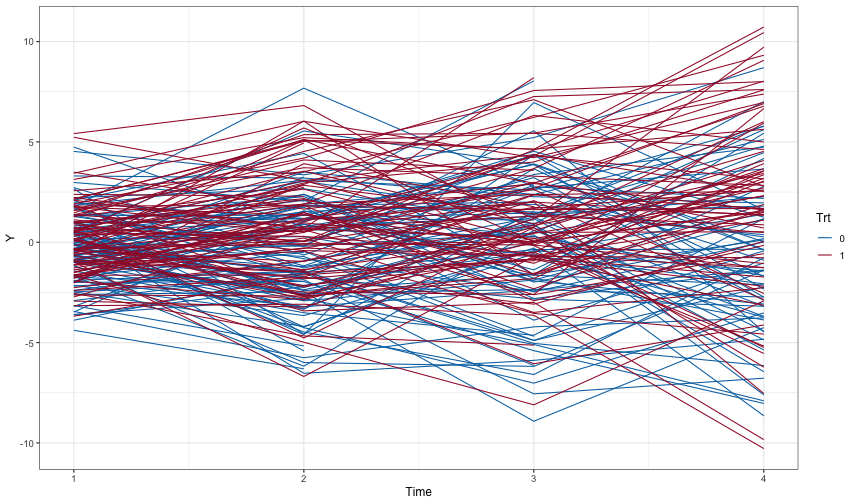
fit0 <- gls(Y~-1+(time1+time2+time3+time4)+(time1+time2+time3+time4):trt,
    correlation = corCompSymm(form = ~ Time | id),
		weights = varIdent(form = ~ 1 | Time),
		data=dd1)
summary(fit0)$tTable
## Value Std.Error t-value p-value
## time1 -0.2498166 0.1857705 -1.3447591 0.1791507428
## time2 -0.7536542 0.2990315 -2.5203167 0.0119523869
## time3 -0.3253077 0.3665450 -0.8874973 0.3751245442
## time4 -0.8114158 0.4966029 -1.6339329 0.1027351197
## time1:trt 0.2980273 0.2627192 1.1343948 0.2570281140
## time2:trt 1.5625956 0.4238492 3.6866786 0.0002452827
## time3:trt 1.3327856 0.5136924 2.5945205 0.0096761138
## time4:trt 2.7390980 0.6883514 3.9792145 0.0000765598fit1 <- gls(Y~-1+time*Trt,
correlation = corCompSymm(form = ~ Time | id),
weights = varIdent(form = ~ 1 | Time),
data=dd1)
(ctrast <- contrast(fit1,
list(time=levels(dd1$time), Trt=levels(dd1$Trt)[2]),
list(time=levels(dd1$time), Trt=levels(dd1$Trt)[1])))## gls model parameter contrast
##
## Contrast S.E. Lower Upper t df Pr(>|t|)
## 0.2980273 0.2627192 -0.2178097 0.8138643 1.13 681 0.2570
## 1.5625955 0.4238486 0.7303884 2.3948025 3.69 681 0.0002
## 1.3327868 0.5136948 0.3241710 2.3414027 2.59 681 0.0097
## 2.7390986 0.6883513 1.3875528 4.0906444 3.98 681 0.0001newdat <- rbind(
with(contrast(fit1, list(time=levels(dd1$time), Trt=levels(dd1$Trt)[1])),
data.frame(time = time, Trt = Trt, Estimate = Contrast, SE = SE,
Lower = Lower, Upper = Upper, 't-value' = testStat, 'p-value' = Pvalue)
),
with(contrast(fit1, list(time=levels(dd1$time), Trt=levels(dd1$Trt)[2])),
data.frame(time = time, Trt = Trt, Estimate = Contrast, SE = SE,
Lower = Lower, Upper = Upper, 't-value' = testStat, 'p-value' = Pvalue)
)
)
newdat$Time <- as.numeric(newdat$time)
ggplot(newdat, aes(y=Estimate, x=Time, color = Trt)) +
geom_smooth(aes(ymax = Upper, ymin = Lower), stat = 'identity')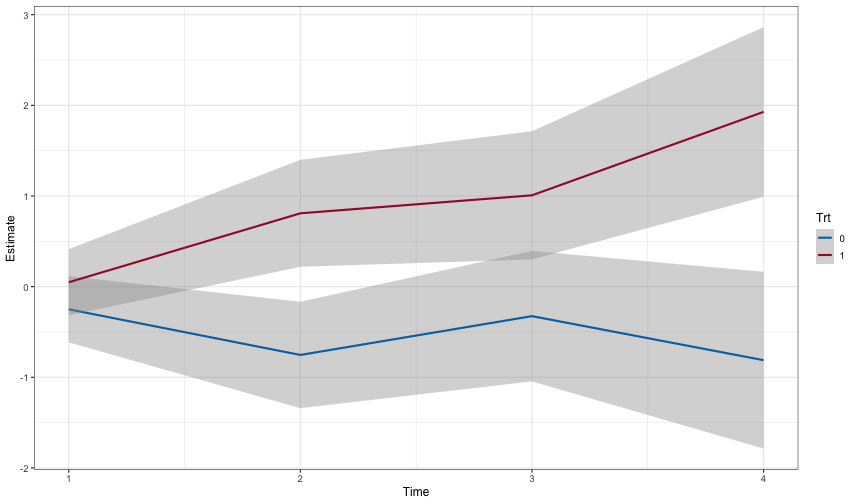
Simulate using parallel
set.seed(20130318)
results <- mclapply(1:10000, function(x){
	dd1 <- merge(dd0, data.frame(id = 1:N, drop = sample(1:5, N, replace=TRUE, p=c(0,0.1,0.1,0.1,0.7))))
	dd1$e <- as.numeric(t(rmvnorm(n=N, mean=rep(0,4), sigma=gls_sigma^2*diag(gls_weights)%*%R%*%diag(gls_weights))))
	dd1$Y <- with(dd1, Y0 + e)
	dd1 <- subset(dd1, Time < drop)
	try(summary(update(fit0, data = dd1))$tTable['time4:trt', 'p-value'], silent = TRUE)
}, mc.cores = 10)
Simulated power results
cat(sum(results < 0.05)/length(results)*100)## 79.99