Constrained Longitudinal Data Analysis

Liang and Zeger (2000) describe a constrained longitudinal data analysis for comparing the time course of two randomized groups in which the model constains the two groups to share a common mean at baseline. Lu (2010) compared the power of this approach to a longitudinal analysis of covariance approach. We conduct a few simple simulation studies to interrogate the effect of the constraint on power to detect group differences. We do not simulate any missing data here.

Packages used

library(longpower)
library(nlme)
library(mvtnorm)
library(parallel)
library(ggplot2)
library(contrast)
library(tidyr)
library(dplyr)

Pre-post design with two repeated measures simulated via random intercept model

Simulation settings

sigma_residual <- 1
sigma_random_intercept <- 1
sigma_random_slope <- 0
Time <- 0:1
Beta <- c('(Intercept)'=1, time=0.5, 'trt:time'=0.4)
Beta.null <- c('(Intercept)'=1, time=0.5, 'trt:time'=0)
n <- 200 # per group
N <- 2*n

Analytic calculations

cov.t <- function(t1, t2, sig2.i, sig2.s, cov.s.i){
        sig2.i + t1*t2*sig2.s + (t1+t2)*cov.s.i
}
m = length(Time)
R = outer(Time, Time, function(x,y){cov.t(x,y, sigma_random_intercept^2, sigma_random_slope^2, 0)})
R = R + diag(sigma_residual^2, m, m)

power.t.test(n=n, delta=Beta['trt:time'], sd=sqrt(2*sigma_random_intercept))


     Two-sample t test power calculation 

              n = 200
          delta = 0.4
             sd = 1.414214
      sig.level = 0.05
          power = 0.8055549
    alternative = two.sided

NOTE: n is number in *each* group

lmmpower(n=n, delta=Beta['trt:time'], t=Time, 
  sig2.e=sigma_residual^2, sig2.s=sigma_random_slope^2, 
  sig2.i=sigma_random_intercept, cov.s.i=0)


     Longitudinal linear model slope power calculation (Diggle et al 2002, page 29) 

              N = 400
              n = 200, 200
          delta = 0.4
         sigma2 = 1
      sig.level = 0.05
          power = 0.8074296
    alternative = two.sided

 NOTE: N is *total* sample size and n is sample size in *each* group 

 R:
     [,1] [,2]
[1,]    2    1
[2,]    1    2

diggle.linear.power(n=n, delta=Beta['trt:time'], t=Time, R=R)


     Longitudinal linear model slope power calculation (Diggle et al 2002, page 29) 

              N = 400
              n = 200, 200
          delta = 0.4
         sigma2 = 1
      sig.level = 0.05
          power = 0.8074296
    alternative = two.sided

 NOTE: N is *total* sample size and n is sample size in *each* group 

 R:
     [,1] [,2]
[1,]    2    1
[2,]    1    2

Set up data for simulation

dd0 <- expand.grid(time = Time, id = 1:N)
dd0$trt <- ifelse(dd0$id <= N/2, 0, 1)
dd0 <- as.data.frame(model.matrix(~ id+trt*time, data = dd0))
dd0$Trt <- as.factor(dd0$trt)
dd0$Y0 <- as.matrix(dd0[, names(Beta)]) %*% Beta
dd0$Y0.null <- as.matrix(dd0[, names(Beta.null)]) %*% Beta.null
ggplot(dd0, aes(x=time, y=Y0, color=Trt)) + geom_line()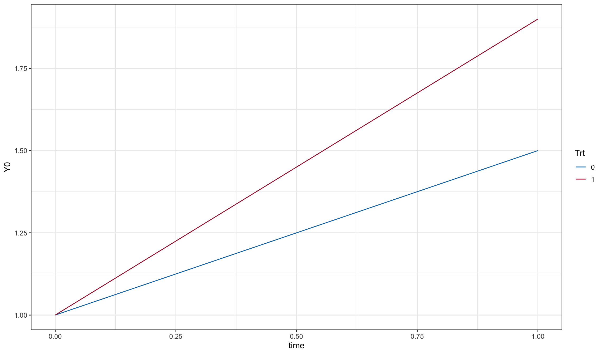

set.seed(20130318)
dd1 <- merge(dd0, data.frame(
  id = 1:N, 
  ran.intercept = rnorm(N, sd=sigma_random_intercept),
  ran.slope     = rnorm(N, sd=sigma_random_slope)
))
dd1$e <- rnorm(nrow(dd1), sd=sigma_residual)

dd1$Y <- with(dd1, Y0 + ran.intercept + ran.slope*time + e)
ggplot(dd1, aes(x=time, y=Y, color=Trt, group = id)) + geom_line()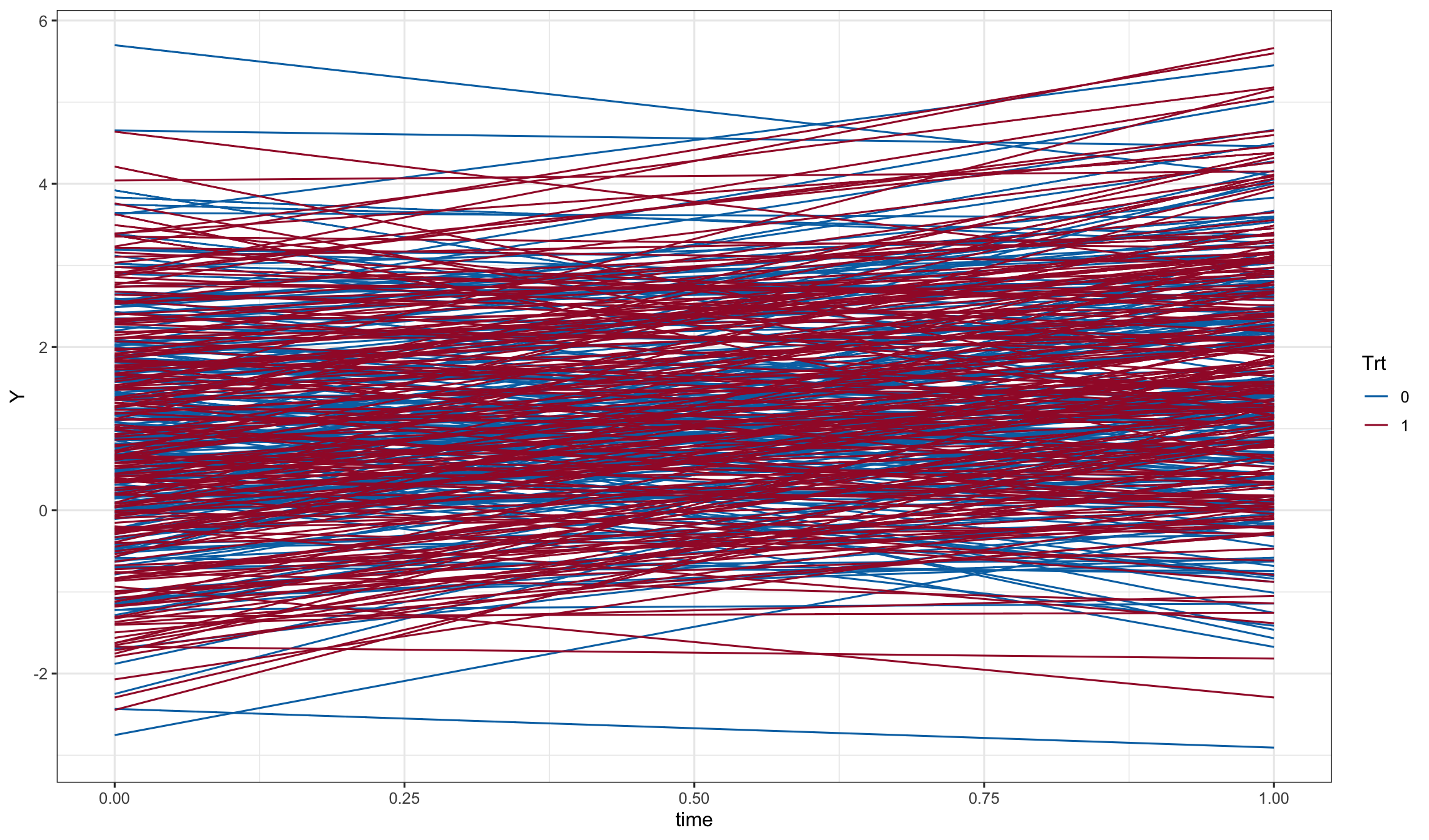

# unconstrained:
fit.LDA <- lme(Y~trt*time, random=~1|id, data=dd1)
printCoefmat(summary(fit.LDA)$tTable)

                 Value  Std.Error         DF t-value   p-value    
(Intercept)   0.994529   0.101708 398.000000  9.7783 < 2.2e-16 ***
trt          -0.172352   0.143837 398.000000 -1.1982  0.231533    
time          0.481055   0.097516 398.000000  4.9331 1.191e-06 ***
trt:time      0.450842   0.137908 398.000000  3.2692  0.001173 ** 
---
Signif. codes:  0 '***' 0.001 '**' 0.01 '*' 0.05 '.' 0.1 ' ' 1

# constrained:
fit.cLDA <- lme(Y~time+time:trt, random=~1|id, data=dd1)
printCoefmat(summary(fit.cLDA)$tTable)

                 Value  Std.Error         DF t-value   p-value    
(Intercept)   0.908353   0.071944 399.000000 12.6259 < 2.2e-16 ***
time          0.520646   0.091756 398.000000  5.6742 2.686e-08 ***
time:trt      0.371660   0.121052 398.000000  3.0703  0.002285 ** 
---
Signif. codes:  0 '***' 0.001 '**' 0.01 '*' 0.05 '.' 0.1 ' ' 1

newdat0 <- expand.grid(trt=0:1, time=Time)

mods <- list(LDA = fit.LDA, cLDA=fit.cLDA)

pd <- do.call(rbind, lapply(names(mods), function(name){
  cbind(newdat0, 
    Y=predict(mods[[name]], newdat0, level=0),
    model = name
  ) 
}))
pd$Trt <- as.factor(pd$trt)
ggplot(pd, aes(y=Y, x=time, color = Trt)) + geom_line() + facet_grid(.~model)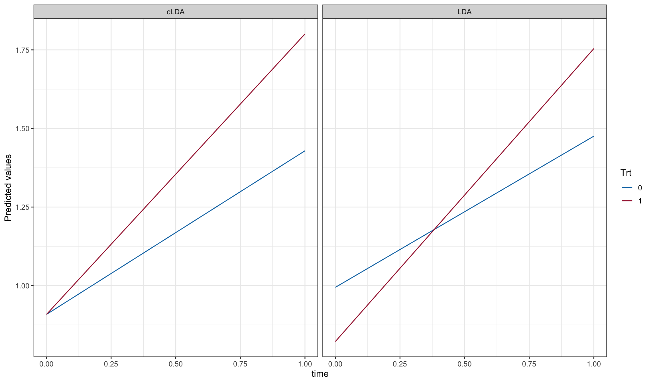

Simulate

set.seed(20130318)
results <- do.call(rbind, mclapply(1:10000, function(x){
  dd1 <- merge(dd0, data.frame(
    id = 1:N,
    ran.intercept = rnorm(N, sd=sigma_random_intercept),
    ran.slope     = rnorm(N, sd=sigma_random_slope)
  ))
  dd1$e <- rnorm(nrow(dd1), sd=sigma_residual)
  dd1$Y <- with(dd1, Y0 + ran.intercept + ran.slope*time + e)
  dd1$Y.null <- with(dd1, Y0.null + ran.intercept + ran.slope*time + e)
  ddw <- merge(
    subset(dd1, time==0, c('id', 'trt', 'Y', 'Y.null')),
    subset(dd1, time==1, c('id', 'trt', 'Y', 'Y.null')),
    by=c('id', 'trt'), suffixes=c('.0','.1')
  )
  ddw$d <- with(ddw, Y.1-Y.0)
  ddw$d.null <- with(ddw, Y.null.1-Y.null.0)

  prepost <- list(
    ttest.power   = t.test(         d~trt, data=ddw)$p.value,
    ttest.alpha   = t.test(    d.null~trt, data=ddw)$p.value,
    ancova1.power = summary(lm(     d~Y.0 + trt, data=ddw))$coef['trt', 'Pr(>|t|)'],
    ancova1.alpha = summary(lm(d.null~Y.null.0 + trt, data=ddw))$coef['trt', 'Pr(>|t|)'],
    ancova2.power = summary(lm(     d~scale(Y.0)*trt, data=ddw))$coef['trt', 'Pr(>|t|)'],
    ancova2.alpha = summary(lm(d.null~scale(Y.null.0)*trt, data=ddw))$coef['trt', 'Pr(>|t|)']
  )

  fits <- list(
    LDA.power  = lme(     Y~time*trt, random=~1|id, data=dd1),
    LDA.alpha  = lme(Y.null~time*trt, random=~1|id, data=dd1),
    cLDA.power = lme(     Y~time+time:trt, random=~1|id, data=dd1),
    cLDA.alpha = lme(Y.null~time+time:trt, random=~1|id, data=dd1)
  )

  c(unlist(prepost),
    slopes = unlist(lapply(fits, function(fit){
      summary(fit)$tTable['time:trt', 'p-value']
    })),
    contrasts = unlist(lapply(fits[1:2], function(fit){
      pv <- try(as.numeric(contrast(fit,
        a=list(time=Time[length(Time)], trt=0),
        b=list(time=Time[length(Time)], trt=1))$Pvalue), silent = TRUE)
      if(class(pv) == 'try-error'){
        fit <- update(fit, random=~1|id)
        pv <- try(as.numeric(contrast(fit,
          a=list(time=Time[length(Time)], trt=0),
          b=list(time=Time[length(Time)], trt=1))$Pvalue), silent = TRUE)
      }
      pv
    }))
  )
}, mc.cores = 10))

Simulated power results (%)

knitr::kable(cbind('Pr(p<0.05)'=apply(results, 2, function(x){
  sum(x < 0.05)/length(x)*100
})))

	Pr(p<0.05)
ttest.power	80.28
ttest.alpha	4.79
ancova1.power	90.15
ancova1.alpha	5.14
ancova2.power	90.15
ancova2.alpha	5.13
slopes.LDA.power	80.28
slopes.LDA.alpha	4.79
slopes.cLDA.power	90.32
slopes.cLDA.alpha	5.15
contrasts.LDA.power	80.56
contrasts.LDA.alpha	5.40

Four repeated measures simulated via random slope model

Simulation settings

sigma_residual <- 1
sigma_random_intercept <- 1
sigma_random_slope <- 1
Time <- 0:3
Beta <- c('(Intercept)'=1, time=0.5, 'trt:time'=0.434)
Beta.null <- c('(Intercept)'=1, time=0.5, 'trt:time'=0)
n <- 100 # per group
N <- 2*n

Analytic calculations

m = length(Time)
R = outer(Time, Time, function(x,y){cov.t(x,y, sigma_random_intercept^2, sigma_random_slope^2, 0)})
R = R + diag(sigma_residual^2, m, m)

lmmpower(n=n, delta=Beta['trt:time'], t=Time, 
  sig2.e=sigma_residual^2, sig2.s=sigma_random_slope^2, 
  sig2.i=sigma_random_intercept^2, cov.s.i=0)


     Longitudinal linear model slope power calculation (Diggle et al 2002, page 29) 

              N = 200
              n = 100, 100
          delta = 0.434
         sigma2 = 1
      sig.level = 0.05
          power = 0.7999644
    alternative = two.sided

 NOTE: N is *total* sample size and n is sample size in *each* group 

 R:
     [,1] [,2] [,3] [,4]
[1,]    2    1    1    1
[2,]    1    3    3    4
[3,]    1    3    6    7
[4,]    1    4    7   11

diggle.linear.power(n=n, delta=Beta['trt:time'], t=Time, R=R)


     Longitudinal linear model slope power calculation (Diggle et al 2002, page 29) 

              N = 200
              n = 100, 100
          delta = 0.434
         sigma2 = 1
      sig.level = 0.05
          power = 0.7999644
    alternative = two.sided

 NOTE: N is *total* sample size and n is sample size in *each* group 

 R:
     [,1] [,2] [,3] [,4]
[1,]    2    1    1    1
[2,]    1    3    3    4
[3,]    1    3    6    7
[4,]    1    4    7   11

Set up data for simulation

dd0 <- expand.grid(time = Time, id = 1:N)
dd0$trt <- ifelse(dd0$id <= N/2, 0, 1)
dd0$t <- as.factor(dd0$time)
dd0 <- as.data.frame(model.matrix(~ id+trt*time+t, data = dd0))
dd0$t <- as.factor(dd0$time)
dd0$Trt <- as.factor(dd0$trt)
dd0$Y0 <- as.matrix(dd0[, names(Beta)]) %*% Beta
dd0$Y0.null <- as.matrix(dd0[, names(Beta.null)]) %*% Beta.null

ggplot(dd0, aes(x=time, y=Y0, color=Trt)) + geom_line()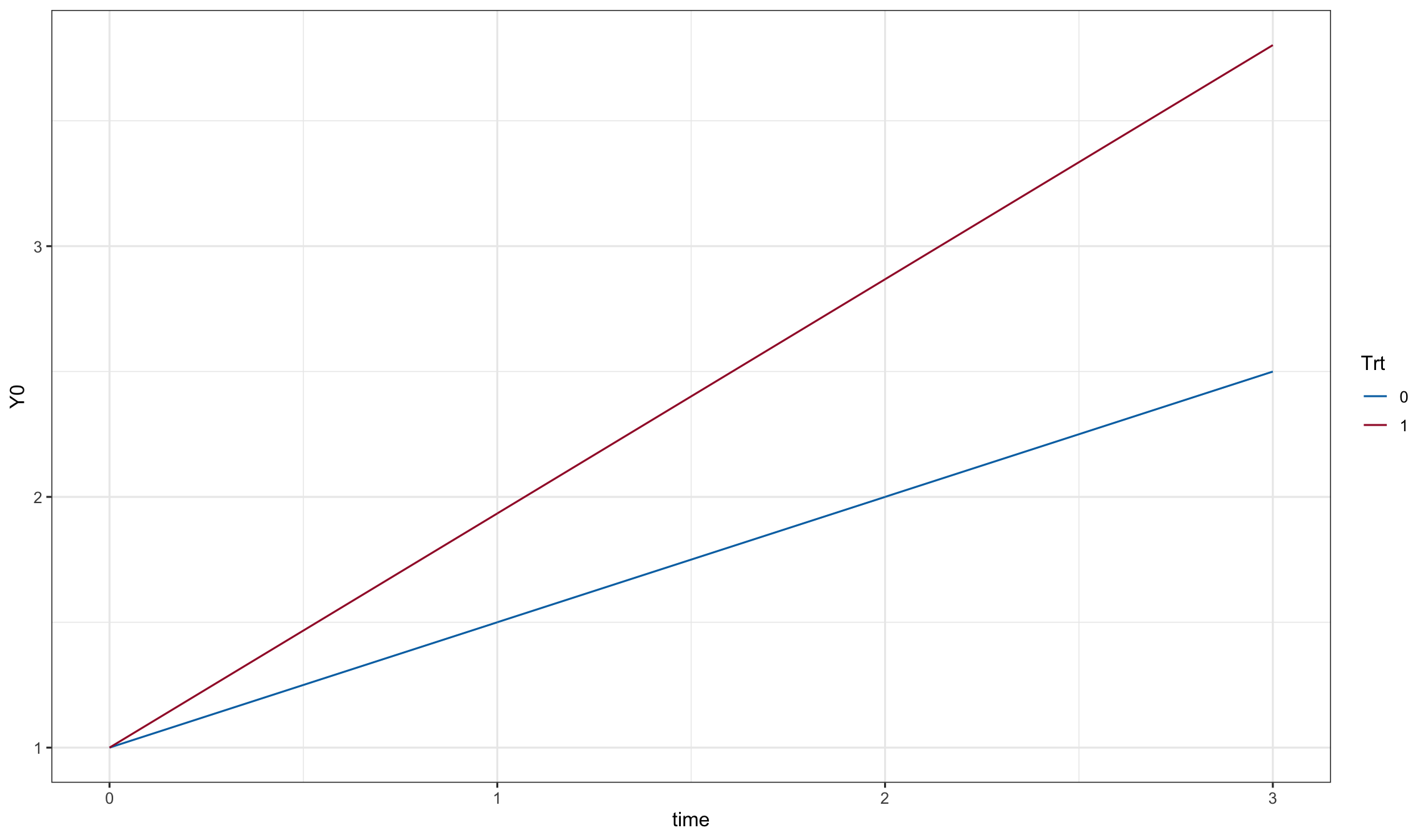

set.seed(20130318)
dd1 <- merge(dd0, data.frame(
  id = 1:N, 
  ran.intercept = rnorm(N, sd=sigma_random_intercept),
  ran.slope     = rnorm(N, sd=sigma_random_slope)
))
dd1$e <- rnorm(nrow(dd1), sd=sigma_residual)

dd1$Y <- with(dd1, Y0 + ran.intercept + ran.slope*time + e)
ggplot(dd1, aes(x=time, y=Y, color=Trt, group = id)) + geom_line()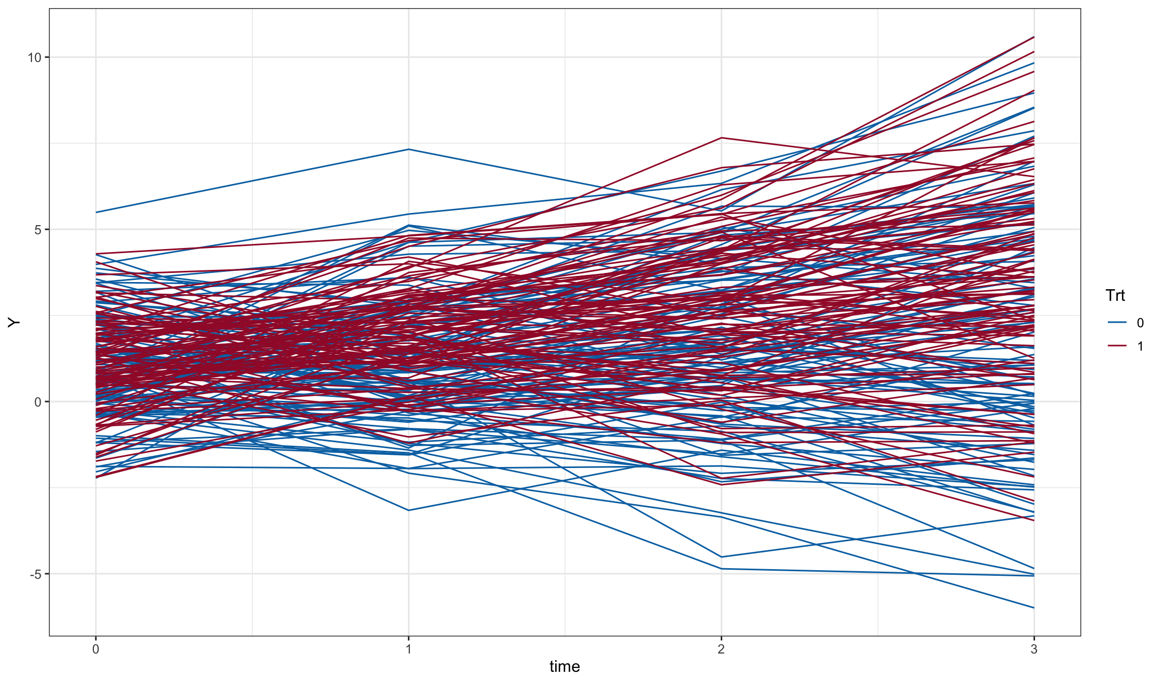

# unconstrained:
fit.LDA <- lme(Y~trt*time, random=~time|id, data=dd1)
printCoefmat(summary(fit.LDA)$tTable)

                Value Std.Error        DF t-value   p-value    
(Intercept)   0.94916   0.13384 598.00000  7.0919 3.749e-12 ***
trt           0.14495   0.18928 198.00000  0.7658  0.444712    
time          0.31195   0.11256 598.00000  2.7714  0.005755 ** 
trt:time      0.48156   0.15918 598.00000  3.0251  0.002592 ** 
---
Signif. codes:  0 '***' 0.001 '**' 0.01 '*' 0.05 '.' 0.1 ' ' 1

# constrained:
fit.cLDA <- lme(Y~time+time:trt, random=~time|id, data=dd1)
printCoefmat(summary(fit.cLDA)$tTable)

                 Value  Std.Error         DF t-value   p-value    
(Intercept)   1.021636   0.094539 598.000000 10.8065 < 2.2e-16 ***
time          0.290433   0.108989 598.000000  2.6648 0.0079117 ** 
time:trt      0.524594   0.148934 598.000000  3.5223 0.0004604 ***
---
Signif. codes:  0 '***' 0.001 '**' 0.01 '*' 0.05 '.' 0.1 ' ' 1

newdat0 <- expand.grid(trt=0:1, time=Time)

mods <- list(LDA = fit.LDA, cLDA=fit.cLDA)

pd <- do.call(rbind, lapply(names(mods), function(name){
  cbind(newdat0, 
    Y=predict(mods[[name]], newdat0, level=0),
    model = name
  ) 
}))
pd$Trt <- as.factor(pd$trt)
ggplot(pd, aes(y=Y, x=time, color = Trt)) + geom_line() + facet_grid(.~model)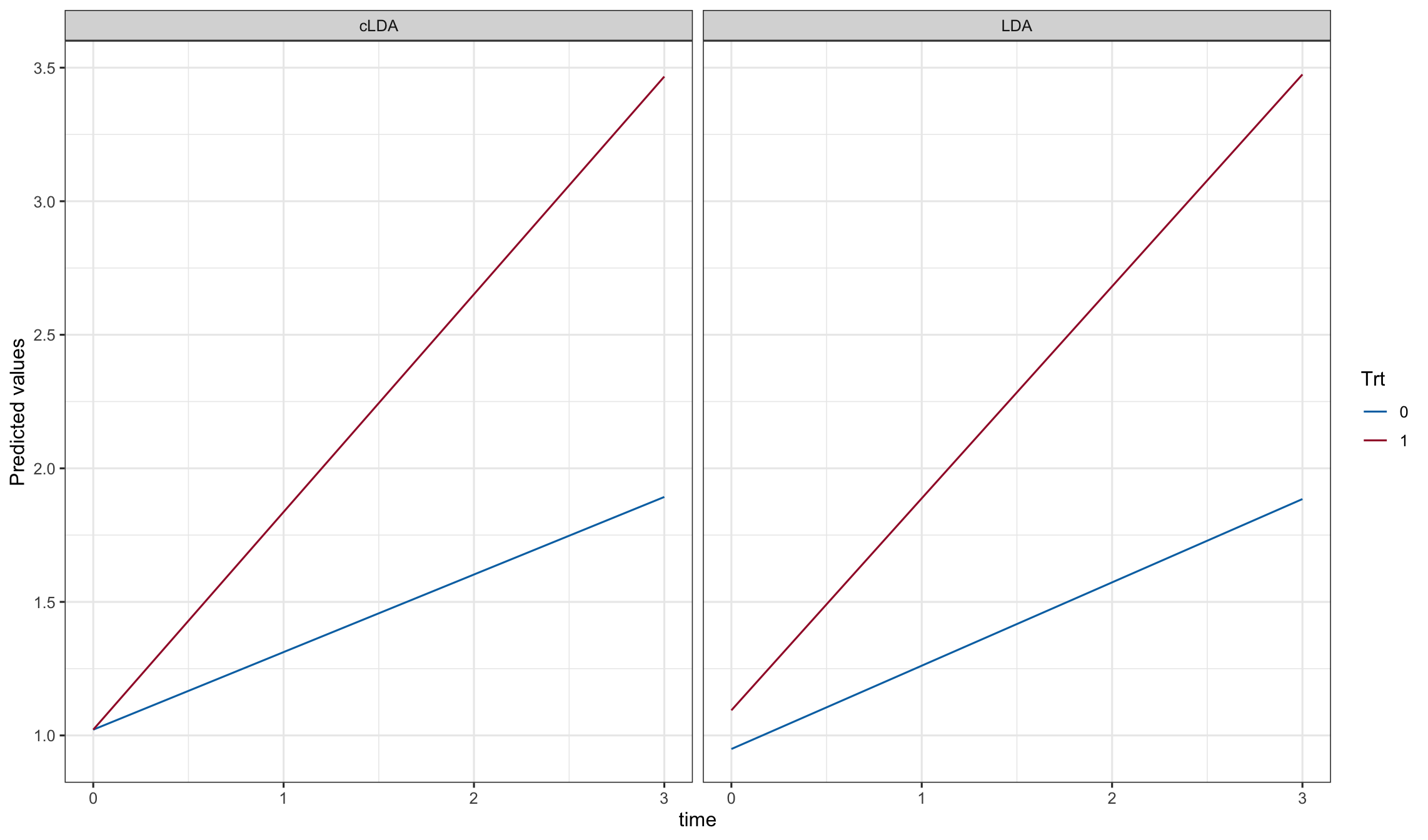

Simulate

set.seed(20130318)
results <- do.call(rbind, mclapply(1:10000, function(x){
  dd1 <- merge(dd0, data.frame(
    id = 1:N,
    ran.intercept = rnorm(N, sd=sigma_random_intercept),
    ran.slope     = rnorm(N, sd=sigma_random_slope)
  ))
  dd1$e <- rnorm(nrow(dd1), sd=sigma_residual)
  dd1$Y <- with(dd1, Y0 + ran.intercept + ran.slope*time + e)
  dd1$Y.null <- with(dd1, Y0.null + ran.intercept + ran.slope*time + e)

  fits.cts <- list(
    LDA.power  = lme(     Y~time*trt, random=~time|id, data=dd1, control=lmeControl(returnObject=TRUE)),
    LDA.alpha  = lme(Y.null~time*trt, random=~time|id, data=dd1, control=lmeControl(returnObject=TRUE)),
    cLDA.power = lme(     Y~time+time:trt, random=~time|id, data=dd1, control=lmeControl(returnObject=TRUE)),
    cLDA.alpha = lme(Y.null~time+time:trt, random=~time|id, data=dd1, control=lmeControl(returnObject=TRUE))
  )

  fits.cat <- list(
    LDA.power  = gls(     Y~(t1+t2+t3)*trt, data=dd1,
      correlation = corCompSymm(form = ~ time | id), weights = varIdent(form = ~ 1 | time)),
    LDA.alpha  = gls(Y.null~(t1+t2+t3)*trt, data=dd1,
      correlation = corCompSymm(form = ~ time | id), weights = varIdent(form = ~ 1 | time)),
    cLDA.power = gls(     Y~t1+t2+t3+(t1+t2+t3):trt, data=dd1,
      correlation = corCompSymm(form = ~ time | id), weights = varIdent(form = ~ 1 | time)),
    cLDA.alpha = gls(Y.null~t1+t2+t3+(t1+t2+t3):trt, data=dd1,
      correlation = corCompSymm(form = ~ time | id), weights = varIdent(form = ~ 1 | time))
  )

  c(slopes = unlist(lapply(fits.cts, function(fit){
      summary(fit)$tTable['time:trt', 'p-value']
    })),
    contrasts.cts = unlist(lapply(fits.cts[1:2], function(fit){
      pv <- try(as.numeric(contrast(fit,
        a=list(time=Time[length(Time)], trt=0),
        b=list(time=Time[length(Time)], trt=1))$Pvalue), silent = TRUE)
      if(class(pv) == 'try-error'){
        fit <- update(fit, random=~1|id)
        pv <- try(as.numeric(contrast(fit,
          a=list(time=Time[length(Time)], trt=0),
          b=list(time=Time[length(Time)], trt=1))$Pvalue), silent = TRUE)
      }
      pv
    })),
    contrasts.cat = c(
      unlist(lapply(fits.cat[1:2], function(fit){
        pv <- try(as.numeric(contrast(fit,
          a=list(t1=0, t2=0, t3=1, trt=0),
          b=list(t1=0, t2=0, t3=1, trt=1))$Pvalue), silent = TRUE)
        pv
      })),
      unlist(lapply(fits.cat[3:4], function(fit){
        summary(fit)$tTable['t3:trt', 'p-value']
      }))
    )
  )
}, mc.cores = 10))

Simulated power results (%)

knitr::kable(cbind('Pr(p<0.05)'=apply(results, 2, function(x){
  sum(x < 0.05)/length(x)*100
})))

	Pr(p<0.05)
slopes.LDA.power	79.74
slopes.LDA.alpha	5.03
slopes.cLDA.power	81.65
slopes.cLDA.alpha	5.08
contrasts.cts.LDA.power	81.12
contrasts.cts.LDA.alpha	5.96
contrasts.cat.LDA.power	81.09
contrasts.cat.LDA.alpha	5.51
contrasts.cat.cLDA.power	87.53
contrasts.cat.cLDA.alpha	10.93

Pre-post design simulated with fixed variance of pre-post difference and various pre-post correlations

Simulation settings

Time <- 0:1
Beta <- c('(Intercept)'=1, time=0.0514, 'trt:time'=0.0514*0.30)
Beta.null <- c('(Intercept)'=1, time=0.0514, 'trt:time'=0)
corr <- c(0.2, 0.5, 0.7)
n <- 64 # per group
N <- 2*n
sd_diff <- 0.0309

Analytic calculations

power.t.test(n=n, delta=Beta['trt:time'], sd=sd_diff)


     Two-sample t test power calculation 

              n = 64
          delta = 0.01542
             sd = 0.0309
      sig.level = 0.05
          power = 0.7999361
    alternative = two.sided

NOTE: n is number in *each* group

Set up data for simulation

dd0 <- expand.grid(time = Time, id = 1:N)
dd0$trt <- ifelse(dd0$id <= N/2, 0, 1)
dd0 <- as.data.frame(model.matrix(~ id+trt*time, data = dd0))
dd0$Trt <- as.factor(dd0$trt)
dd0$Y0 <- as.matrix(dd0[, names(Beta)]) %*% Beta
dd0$Y0.null <- as.matrix(dd0[, names(Beta.null)]) %*% Beta.null

Simulate

set.seed(20130318)
results <- do.call(rbind, mclapply(1:10000, function(x){
  ll <- lapply(corr, function(rho){
    sd_resid <- sqrt(sd_diff^2/(2*(1-rho)))
    cov_resid <- rho * sd_resid^2
    resids <- gather(
      data.frame(
        id = 1:N,
        rmvnorm(n=N, mean=c(0,0), sigma=matrix(c(sd_resid^2,cov_resid,cov_resid,sd_resid^2), nrow=2))), 
      time, e, 2:3) %>% 
      mutate(time = as.numeric(gsub('X', '', time))-1)
    dd1 <- merge(dd0, resids, by=c('id', 'time'))
    dd1$Y <- with(dd1, Y0 + e)
    dd1$Y.null <- with(dd1, Y0.null + e)
    ddw <- merge(
      subset(dd1, time==0, c('id', 'trt', 'Y', 'Y.null')),
      subset(dd1, time==1, c('id', 'trt', 'Y', 'Y.null')),
      by=c('id', 'trt'), suffixes=c('.0','.1')
    )
    ddw$d <- with(ddw, Y.1-Y.0)
    ddw$d.null <- with(ddw, Y.null.1-Y.null.0)

    prepost <- list(
      ttest.power   = t.test(         d~trt, data=ddw)$p.value,
      ttest.alpha   = t.test(    d.null~trt, data=ddw)$p.value,
      ancova1.power = summary(lm(     d~Y.0 + trt, data=ddw))$coef['trt', 'Pr(>|t|)'],
      ancova1.alpha = summary(lm(d.null~Y.null.0 + trt, data=ddw))$coef['trt', 'Pr(>|t|)'],
      ancova2.power = summary(lm(     d~scale(Y.0)*trt, data=ddw))$coef['trt', 'Pr(>|t|)'],
      ancova2.alpha = summary(lm(d.null~scale(Y.null.0)*trt, data=ddw))$coef['trt', 'Pr(>|t|)']
    )

    fits <- list(
      LDA.power  = lme(     Y~time*trt, random=~1|id, data=dd1, control=lmeControl(returnObject=TRUE)),
      LDA.alpha  = lme(Y.null~time*trt, random=~1|id, data=dd1, control=lmeControl(returnObject=TRUE)),
      cLDA.power = lme(     Y~time+time:trt, random=~1|id, data=dd1, control=lmeControl(returnObject=TRUE)),
      cLDA.alpha = lme(Y.null~time+time:trt, random=~1|id, data=dd1, control=lmeControl(returnObject=TRUE))
    )

    c(unlist(prepost),
      slopes = unlist(lapply(fits, function(fit){
        summary(fit)$tTable['time:trt', 'p-value']
      })),
      contrasts = unlist(lapply(fits[1:2], function(fit){
        pv <- try(as.numeric(contrast(fit,
          a=list(time=Time[length(Time)], trt=0),
          b=list(time=Time[length(Time)], trt=1))$Pvalue), silent = TRUE)
        if(class(pv) == 'try-error'){
          fit <- update(fit, random=~1|id)
          pv <- try(as.numeric(contrast(fit,
            a=list(time=Time[length(Time)], trt=0),
            b=list(time=Time[length(Time)], trt=1))$Pvalue), silent = TRUE)
        }
        pv
      }))
    )
  })
  names(ll) <- corr
  unlist(ll)
}, mc.cores = 10))

Simulated power results (%)

knitr::kable(cbind('Pr(p<0.05)'=apply(results, 2, function(x){
  sum(x < 0.05)/length(x)*100
})))

	Pr(p<0.05)
0.2.ttest.power	68.03
0.2.ttest.alpha	4.87
0.2.ancova1.power	58.75
0.2.ancova1.alpha	4.73
0.2.ancova2.power	58.82
0.2.ancova2.alpha	4.73
0.2.slopes.LDA.power	67.97
0.2.slopes.LDA.alpha	4.87
0.2.slopes.cLDA.power	58.13
0.2.slopes.cLDA.alpha	4.85
0.2.contrasts.LDA.power	58.24
0.2.contrasts.LDA.alpha	4.59
0.5.ttest.power	67.45
0.5.ttest.alpha	5.17
0.5.ancova1.power	67.18
0.5.ancova1.alpha	4.97
0.5.ancova2.power	67.29
0.5.ancova2.alpha	4.97
0.5.slopes.LDA.power	67.41
0.5.slopes.LDA.alpha	5.17
0.5.slopes.cLDA.power	67.11
0.5.slopes.cLDA.alpha	5.08
0.5.contrasts.LDA.power	67.42
0.5.contrasts.LDA.alpha	5.03
0.7.ttest.power	67.72
0.7.ttest.alpha	5.02
0.7.ancova1.power	67.82
0.7.ancova1.alpha	5.05
0.7.ancova2.power	67.99
0.7.ancova2.alpha	5.06
0.7.slopes.LDA.power	67.64
0.7.slopes.LDA.alpha	5.02
0.7.slopes.cLDA.power	67.78
0.7.slopes.cLDA.alpha	4.95
0.7.contrasts.LDA.power	55.50
0.7.contrasts.LDA.alpha	5.09

So the t-test power is fixed at 80% (by design), the unconstrained LDA has nearly identical power to t-test; while ANCOVA and constrained LDA have similar power (always better power than t-test, but power decreases with increasing pre-post correlation). ANCOVA2 has similar power as ANCOVA1 (not surprising since no interaction between baseline outcome and group was simulated).

This confirms that the cLDA is preferred whenever we have two timepoints in a randomized study; just as ANCOVA is always preferred to t-test. Of course, cLDA has the added advantage of accommodating missing data.