Power for MMRM

We use the power calculation formula of Lu, Luo and Chen (2008) for Mixed Models of Repeated Measures, which accomodates general missing data patterns. This formula is implemented in the longpower package. We also verify the formula with a simple simulation.

Load packages

library(longpower)
library(nlme)
library(mvtnorm)
library(parallel)
library(ggplot2)
library(contrast)

Simulation settings

gls_sigma <- 2
gls_weights <- c(1, 1.5, 1.75, 2.0)
placebo_mean <- c(0, 0, 0, 0)
active_mean <- c(0, 1, 1.5, 1.8)
retention <- c(1, 0.9, 0.8, 0.7)
# compound symmetric R
R <- matrix(0.5, nrow = 4, ncol = 4)
diag(R) <- 1
N <- 200

Analytic calculations

power.mmrm(power=0.80, ra = retention, Ra=R, N=N, sigmaa = gls_sigma*gls_weights[4])


     Power for Mixed Model of Repeated Measures (Lu, Luo, & Chen, 2008) 

             n1 = 100
             n2 = 100
     retention1 = 1.0, 0.9, 0.8, 0.7
     retention2 = 1.0, 0.9, 0.8, 0.7
          delta = 1.798283
      sig.level = 0.05
          power = 0.8
    alternative = two.sided

power.t.test(power=0.80, n = N/2*retention[4], sd = gls_sigma*gls_weights[4])


     Two-sample t test power calculation 

              n = 70
          delta = 1.907529
             sd = 4
      sig.level = 0.05
          power = 0.8
    alternative = two.sided

NOTE: n is number in *each* group

The t-test delta is larger, which is expect given the conservative handling of the assumed retention rate. The MMRM makes use of partial informatin from dropouts.

Set up data for simulation

dd0 <- expand.grid(time = as.factor(1:4), id = 1:N)
dd0$Time <- as.numeric(dd0$time)
dd0$trt <- ifelse(dd0$id <= N/2, 0, 1)
dd0 <- as.data.frame(model.matrix(~ -1+id+trt*time+Time, data = dd0))
dd0[,'trt:time1'] <- with(dd0, trt*time1)
dd0$Trt <- as.factor(dd0$trt)
dd0$time <- as.factor(dd0$Time)
dd0$Y0[dd0$trt==1] <- as.matrix(subset(dd0, trt==1, c('trt:time1', 'trt:time2', 
  'trt:time3', 'trt:time4'))) %*% active_mean
dd0$Y0[dd0$trt==0] <- as.matrix(subset(dd0, trt==0, c('time1', 'time2', 
  'time3', 'time4'))) %*% placebo_mean
ggplot(dd0, aes(x=Time, y=Y0, color=Trt)) + geom_line()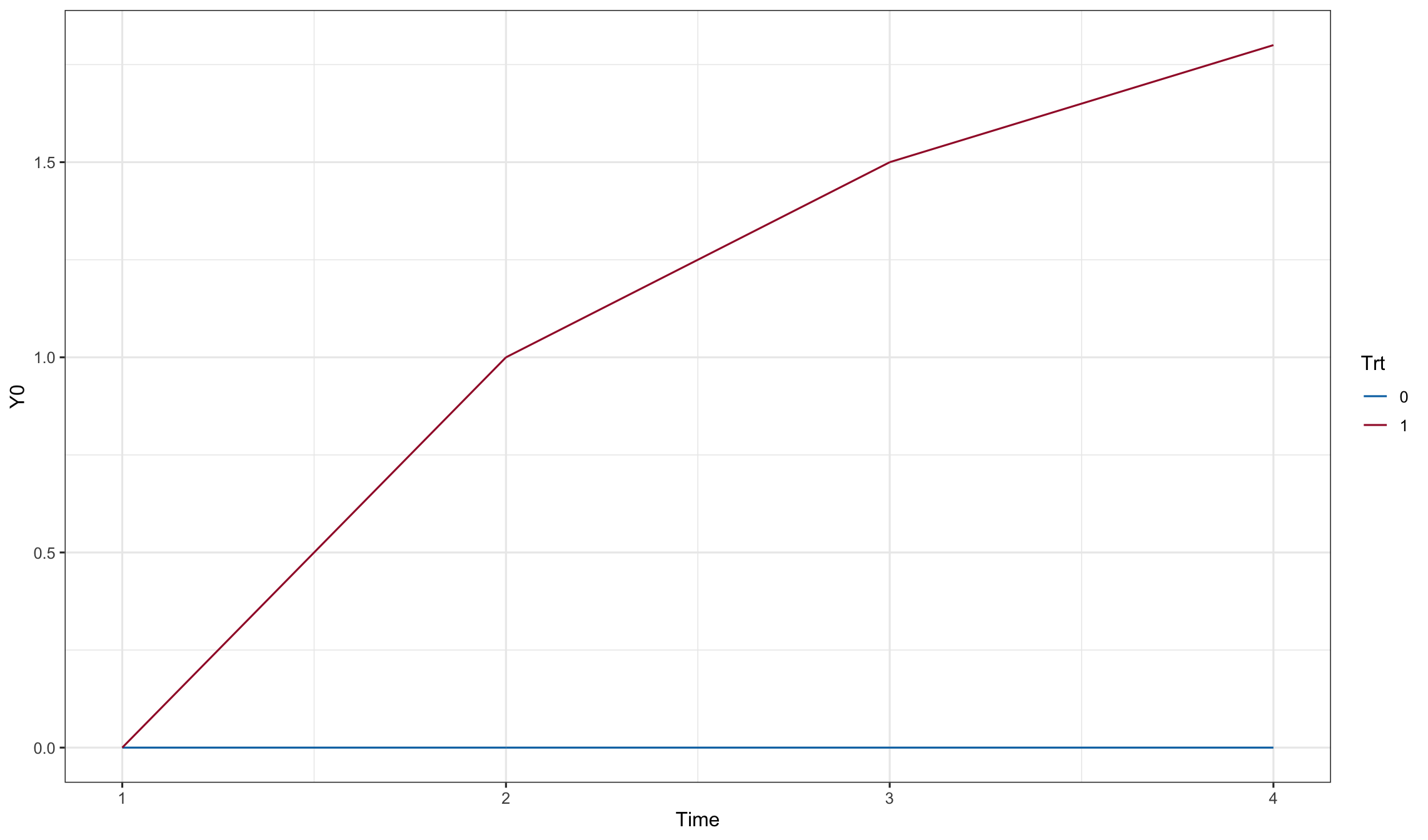

set.seed(20130318)
dd1 <- merge(dd0, data.frame(id = 1:N, drop = sample(1:5, N, replace=TRUE, p=c(0,0.1,0.1,0.1,0.7))))
dd1$e <- as.numeric(t(rmvnorm(n=N, mean=rep(0,4), sigma=gls_sigma^2*diag(gls_weights)%*%R%*%diag(gls_weights))))
dd1$Y <- with(dd1, Y0 + e)
dd1 <- subset(dd1, Time < drop)
ggplot(dd1, aes(x=Time, y=Y, color=Trt, group = id)) + geom_line()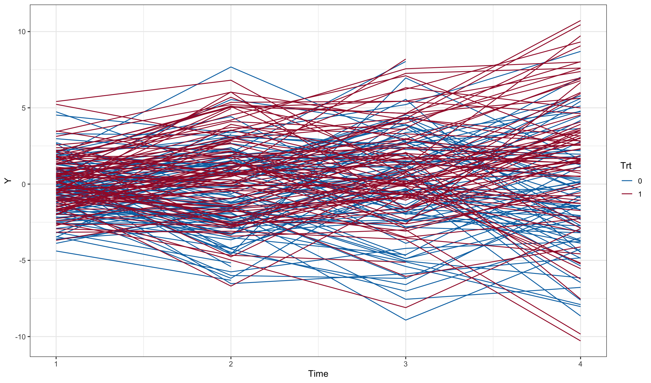

fit0 <- gls(Y~-1+(time1+time2+time3+time4)+(time1+time2+time3+time4):trt, 
    correlation = corCompSymm(form = ~ Time | id),
        weights = varIdent(form = ~ 1 | Time),
        data=dd1)
summary(fit0)$tTable

               Value Std.Error    t-value      p-value
time1     -0.2498166 0.1857705 -1.3447591 0.1791507434
time2     -0.7536542 0.2990315 -2.5203167 0.0119523864
time3     -0.3253077 0.3665450 -0.8874973 0.3751245464
time4     -0.8114158 0.4966029 -1.6339329 0.1027351200
time1:trt  0.2980273 0.2627192  1.1343948 0.2570281147
time2:trt  1.5625956 0.4238492  3.6866786 0.0002452827
time3:trt  1.3327856 0.5136925  2.5945204 0.0096761153
time4:trt  2.7390980 0.6883514  3.9792145 0.0000765598

fit1 <- gls(Y~-1+time*Trt, 
  correlation = corCompSymm(form = ~ Time | id),
    weights = varIdent(form = ~ 1 | Time),
    data=dd1)

(ctrast <- contrast(fit1, 
  list(time=levels(dd1$time), Trt=levels(dd1$Trt)[2]),
  list(time=levels(dd1$time), Trt=levels(dd1$Trt)[1])))

gls model parameter contrast

  Contrast      S.E.      Lower     Upper    t  df Pr(>|t|)
 0.2980273 0.2627192 -0.2178097 0.8138642 1.13 681   0.2570
 1.5625955 0.4238486  0.7303884 2.3948026 3.69 681   0.0002
 1.3327868 0.5136947  0.3241710 2.3414026 2.59 681   0.0097
 2.7390986 0.6883513  1.3875528 4.0906444 3.98 681   0.0001

newdat <- rbind(
  with(contrast(fit1, list(time=levels(dd1$time), Trt=levels(dd1$Trt)[1])),
       data.frame(time = time, Trt = Trt, Estimate = Contrast, SE = SE,
                  Lower = Lower, Upper = Upper, 't-value' = testStat, 'p-value' = Pvalue)
       ),
  with(contrast(fit1, list(time=levels(dd1$time), Trt=levels(dd1$Trt)[2])),
       data.frame(time = time, Trt = Trt, Estimate = Contrast, SE = SE,
                  Lower = Lower, Upper = Upper, 't-value' = testStat, 'p-value' = Pvalue)
       )
  )
newdat$Time <- as.numeric(newdat$time)
ggplot(newdat, aes(y=Estimate, x=Time, color = Trt)) +
    geom_smooth(aes(ymax = Upper, ymin = Lower), stat = 'identity')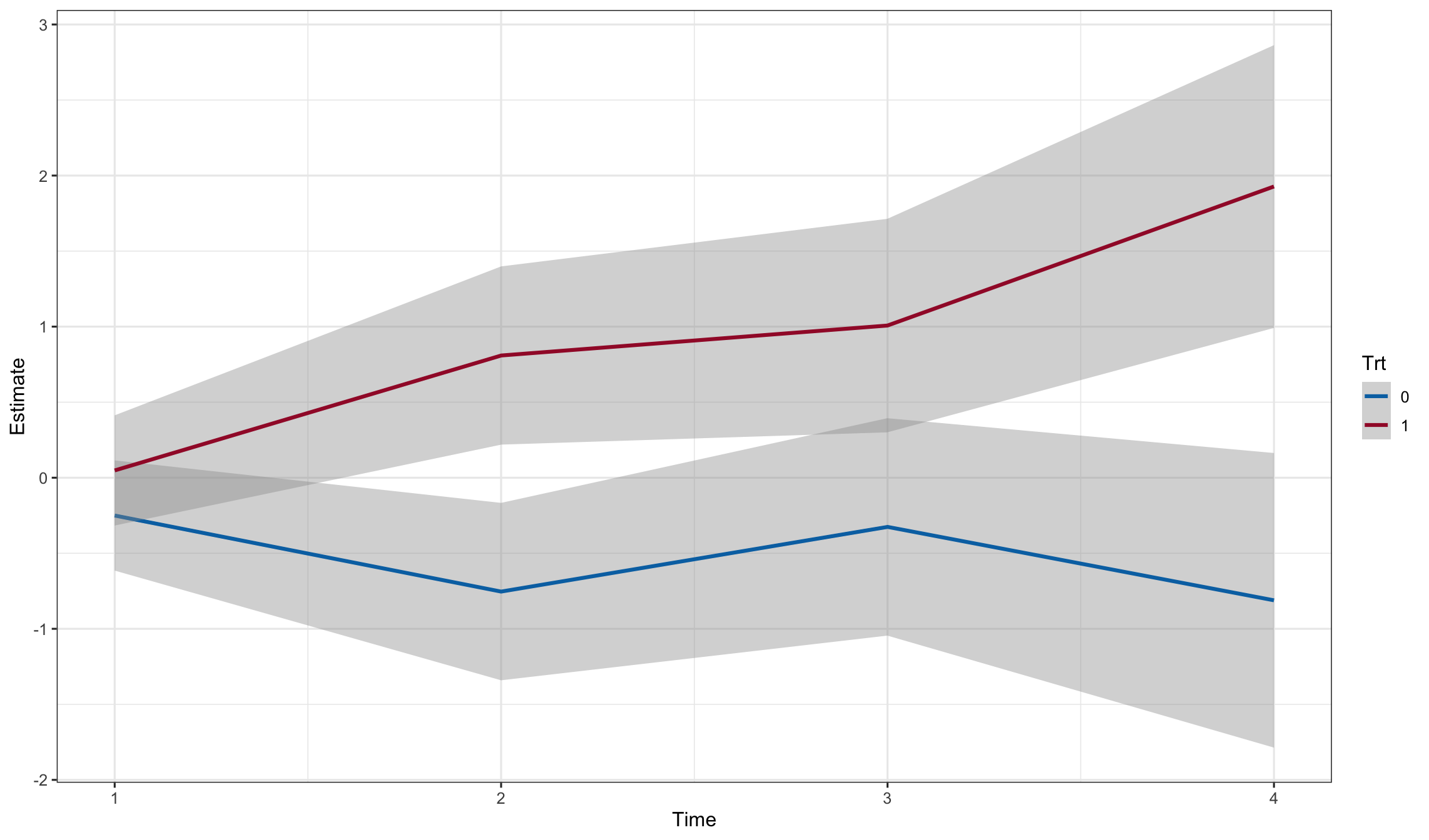

Simulate using parallel

set.seed(20130318)  
results <- mclapply(1:10000, function(x){
    dd1 <- merge(dd0, data.frame(id = 1:N, drop = sample(1:5, N, replace=TRUE, p=c(0,0.1,0.1,0.1,0.7))))
    dd1$e <- as.numeric(t(rmvnorm(n=N, mean=rep(0,4), sigma=gls_sigma^2*diag(gls_weights)%*%R%*%diag(gls_weights))))
    dd1$Y <- with(dd1, Y0 + e)
    dd1 <- subset(dd1, Time < drop)
    try(summary(update(fit0, data = dd1))$tTable['time4:trt', 'p-value'], silent = TRUE)
}, mc.cores = 10)

Simulated power results

cat(sum(results < 0.05)/length(results)*100)

79.99